Learn Programming online

Started Two months Online Programming Classes for XI, XII (all boards), B.Sc.(CS/IT), BCA, M.Sc.(CS/IT), MCA.

Programming Languages

1. C

2. C++

3. Python Basics

4. Python for Data Science

5. R programming

Web Designing

1. HTML

2. CSS

3. PHP

Theory Papers

1. DBMS

2. OS

3. Data Structure using C/C++

New Batches starting from 25 May. Limited Seats. 

Comment Below your contact details(name, email-id and mobile number) if your are interested.

Doubts / Queries

Comment below your queries, doubts or you want to understand any concept related with Data Structure again. 

Heap Sort Algorithm

What is heap?

A heap is defined as a complete binary tree with n nodes such that

1. Value of each node is less than or equal to the root. When root of the binary tree is the biggest number in the heap. This type of heap is known as max Heap  or descending Heap.


2. Value of each node is greater than or equal to the root. When root of the binary tree is the smallest number in the heap. This type of heap is known as min Heap  or ascending Heap.

Each node in the heap corresponds to an element of the array, with the root node corresponding to the element with index 0 in the array. Considering a node corresponding to index i, then its left child has index (2*i + 1) and its right child has index (2*i + 2).

Heap can be used to sort the data in ascending and descending order. The method is known as Heap Sort. Heap Sort involves two basic step

1. Build Heap

•      Create max heap to sort the data in ascending order
•      Create min Heap to sort data in descending order

2. Heapify


ALGORITHM 
    Heapify(A, i){
        l <- left(i)
        r <- right(i)
        if l <= heapsize[A] and A[l] > A[i]
            then largest <- l
            else largest <- i
        if r <= heapsize[A] and A[r] > A[largest]
            then largest <- r
        if largest != i
            then swap A[i] <-> A[largest]
                Heapify(A, largest)
    }

    Buildheap(A){
        heapsize[A] <- length[A]
        for i <- |length[A]/2| downto 1
            do Heapify(A, i)
    }

    Heapsort(A){
        Buildheap(A)
        for i <- length[A] downto 2
            do swap A[1] <-> A[i]
            heapsize[A] <- heapsize[A] - 1
            Heapify(A, 1)
    }

Kruskal Algorithm

DEFINITION - Minimum Cost Spanning Tree

Let G=(V,E,W) be any weighted graph. Then a spanning tree whose cost is minimum is called minimum spanning tree. The cost of the spanning tree is defined as the sum of the costs of the edges in that tree.

Kruskal’s Algorithm

Kruskal’s Algorithm uses greedy approach to select an edge with a minimum cost that doesn't result in cycle when added to already selected edges. Time complexity of Kruskal’s algorithm is o(n+eloge).
In this method all the edges are arranged in the increasing order of the cost. Now select one by one the edges with minimum cost but edges are accepted if and only if there is no cycle. All the other edges having high cost or cycle is formed are rejected.

The steps involved are

Step 1: Construct a min heap of edges on the basis of ascending order of cost of edges.

Step 2: Delete edge from heap and add to minimum cost spanning tree T if no cycle

Step 3: Repeat until e=n-1 or heap is empty

EXAMPLE

Prim's Method

DEFINITION - Minimum Cost Spanning Tree

Let G=(V,E,W) be any weighted graph. Then a spanning tree whose cost is minimum is called minimum spanning tree. The cost of the spanning tree is defined as the sum of the costs of the edges in that tree.

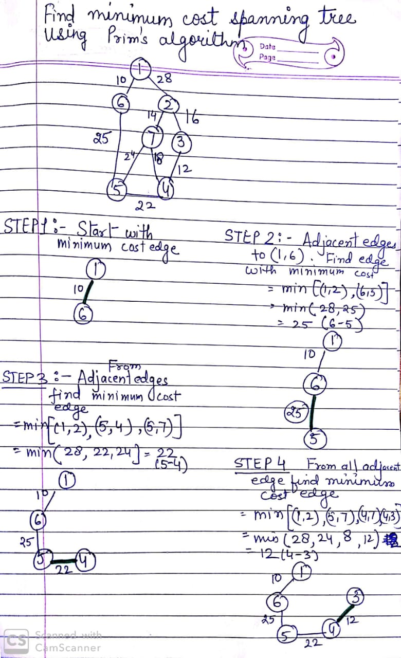
Prim's Algorithm 

In Prim’s algorithm, greedy criterion is used to determine the next edge that have minimum cost. It has a time complexity of O(n²). The steps to find minimum cost spanning tree using Prim’s algorithm is

The steps involved are

Step 1: Select the minimum cost edge and include in minimum spanning tree T

Step 2: Select adjacent edges to T which is minimum in cost and add to T

Step 3: Repeat Step 1 and 2 for n-1 edges and no cycle

EXAMPLE

Introduction of Graphs

A graph consists of two sets V and E.

• V is finite and non empty set of vertices
• E is a set of edges connecting two vertices. 

Graphs can be directed or undirected

Directed Graph: If all the edges of a graph have specific direction then this type of graph is called directed graph.For Example: V = {1,2,3,4} and E={(1,2), (2,3), (2,4), (3,1), (4,1), (4,3)}Then Directed Graph G={V,E} represented as

Undirected Graph: If all the edges of the graphs has no specific direction then this type of graph  is known as undirected graph.For Example: V = {1,2,3,4} and E={(1,2), (1,3),(1,4), (2,1),(2,3),(2,4), (3,1),(3,2),(3,4), (4,1),(4,2), (4,3)}Then Undirected Graph G={V,E} represented as

 Representation of Graph

Adjacency Matrix: It is the two dimensional array or matrix representation of graph. In the matrix, the element a(i,j)= 0 if there is no edge between vertex i and j; the element a(i,j)=1 if there is an edge between vertex i and j. It is also known as Static Representation of graph.

For Example : Consider the following Directed Graph.  The Adjacent Matrix is 

        1    2     3     4

1      0    1     0     0

2      0    0     0     1

3      0    0     0     0

4      1    0     1     0




Consider the following Undirected Graph.  The Adjacent Matrix is  

        1    2     3     4

1      0    1     0     1

2      1    0     0     1

3      0    0     0     0

4      1    1     1     0

Adjacency List: It is the list representation of graphs. In this representation, if there are n vertices then there are n linked list for each vertex of graph. It is also known as Dynamic Representation of graph.

Traversing a Graphs

Exploring each vertex of the graph is known as traversing a graph. The order in which we explored the vertices depend upon what kind of data structure is used.  The two common graph traversal method are

1. Breadth First Search (BFS)
2. Depth First Search (DFS)

Spanning Tree 

A tree T is a spanning tree of a graph G={V,E} if every vertex of G belongs to an edge in T and theedges in T form a tree. Details...

Graph Traversal - Breadth First Search

Breadth First Search can be used to find the shortest distance between some starting vertex and remaining vertex of the graph. In this method, all the vertices are stored in a Queue and each vertex of the graph is visited or explored once. The oldest vertex (added first) in the Queue is explored first. To traverse the graph using breadth first search, Adjacent List of a graph is created first.

EXAMPLE

For Example : Consider the following Graph

The Adjacent List is

11 -> 12,18,13

12-> 11,14,15

13-> 11,16,17

14-> 12,18

15-> 12,18

16-> 13,18

17-> 13,18

18-> 14,15,11,16,17

Let us suppose that starting node is 11, The steps to traverse graph using Breadth First Search Is

Step 1: Add 11 to queue

Front: 1                    Queue: 11

Rear:1

Step 2: Delete element at Front  position (11) and add all the adjacent nodes of deletd not that are not visited.

Front: 2                    Queue: X,12, 18, 13

Rear:4

Step 3: Delete element at Front position (12) and add all the adjacent nodes of deletd not that are not visited.

Front: 3                    Queue: X,X,18, 13, 14, 15           

Rear:6

 11 already visited; i.e. in Queue or deleted

Step 4: Delete element at Front position (18) and add all the adjacent nodes of deletd not that are not visited.

Front: 4                    Queue: X,X,X,13, 14, 15, 16,17        

Rear:8

11,14,15 already visited; i.e. in Queue or deleted

Step 5: Delete element at Front position (13) and add all the adjacent nodes of deletd not that are not visited.

Front: 5                    Queue: X,X,X,X, 14, 15, 16,17        

Rear:8

No vertex added becoz 11,16,17 already visited; i.e. in Queue or deleted

Step 6: Delete element at Front position (14) and add all the adjacent nodes of deletd not that are not visited.

Front: 6                    Queue: X,X,X,X, X, 15, 16,17       

Rear:8

No vertex added becoz 12 and 18 already visited; i.e. in Queue or deleted

Step 7: Delete element at Front position (15) and add all the adjacent nodes of deletd not that are not visited.

Front: 7                    Queue: X,X,X,X, X,X,16,17      

Rear:8

No vertex added becoz 12 and 18 already visited; i.e. in Queue or deleted

Step 8: Delete element at Front position (16) and add all the adjacent nodes of deletd not that are not visited.

Front: 8                    Queue: X,X,X,X, X,X,X,17      

Rear:8

No vertex added becoz 13 and 18 already visited; i.e. in Queue or deleted

Step 9: Delete element at Front position (17) and add all the adjacent nodes of deletd not that are not visited.

Front: 8                   Queue: X,X,X,X, X,X,X,X      

Rear:8

No vertex added becoz 13 and 18 already visited; i.e. in Queue or deleted

Queue EMPTY. STOP.

Therefore Breadth First Search is 11,12,18,13,14,15,16,17

ALGORITHM

Step 1: Initialize all the vertices and create adjacent list.

Step 2: Put Starting vertex in Queue.

Step 3: Repeat Step 4 and 5 until Queue is empty.

Step 4: Remove front node from the Queue.

Step 5: Add to the rear of the Queue all the neighbors of the deleted node that are not visited or added in a Queue.

Step 6: Exit

APPLICATIONS

1. Used to test whether graph is connected or not
2. To find the cycles in the graphs
3. To find the path with minimum number of edges between start vertex and current vertex or reporting that no such path exists.

Graph Traversal - Depth First Search

Depth First Search is used to perform traversal of a graph. In this method, all the vertices are stored in a Stack and each vertex of the graph is visited or explored once. The newest vertex (added last) in the Stack is explored first. To traverse the graph, Adjacent List of a graph is created first.

EXAMPLE

For Example : Consider the following Graph

The Adjacent List is

11 -> 12,18,13

12-> 11,14,15

13-> 11,16,17

14-> 12,18

15-> 12,18

16-> 13,18

17-> 13,18

18-> 14,15,11,16,17

Let us suppose that starting node is 11, The steps to traverse graph using Depth First Search is

Step 1: Push 11 onto the Stack

Stack: 11

Step 2:  Pop the top element i.e. last added (11) from the stack and push all adjacent vertex of popped vertex onto the stack that are not visited.

Stack:  12,18,13

Step 3:  Pop the top element i.e. last added (13) from the stack and push all adjacent vertex of popped vertex onto the stack that are not visited.

Stack: 12,18,16,17

11 not added becoz already visited; i.e. onto stack or deleted

Step 4:  Pop the top element i.e. last added (17) from the stack and push all adjacent vertex of popped vertex onto the stack that are not visited.

Stack: 12,18,16

13 and 18 not added becoz already visited; i.e. onto stack or deleted

Step 5:  Pop the top element i.e. last added (16) from the stack and push all adjacent vertex of popped vertex onto the stack that are not visited.

Stack: 12,18

13 and 18 not added becoz already visited; i.e. onto stack or deleted

Step 6:  Pop the top element i.e. last added (18) from the stack and push all adjacent vertex of popped vertex onto the stack that are not visited.

Stack: 12,14,15

11,16 and 17 not added becoz already visited; i.e. onto stack or deleted

 

Step 7:  Pop the top element i.e. last added (15) from the stack and push all adjacent vertex of popped vertex onto the stack that are not visited.

Stack: 12,14

12 and 18  not added becoz already visited; i.e. onto stack or deleted

Step 8:  Pop the top element i.e. last added (14) from the stack and push all adjacent vertex of popped vertex onto the stack that are not visited.

Stack: 12

12 and 18  not added becoz already visited; i.e. onto stack or deleted

 

Step 9:  Pop the top element i.e. last added (12) from the stack and push all adjacent vertex of popped vertex onto the stack that are not visited.

Stack: ----

11, 14 and 15  not added becoz already visited; i.e. onto stack or deleted

Stack Empty. Therefore the Depth First Search is  11,13,17,16,18, 15,14,12

METHOD

Step 1: Intialise all the vertices.

Step 2: Push starting vertex onto the Stack.

Step 3: Repeat step 4 and 5 until Stack is empty.

Step 4: Pop the top vertex from the Stack.

Step 5: Push onto stack all the neighbours of Popped vertex

Step 6: Exit

ALGORITHM

Step 1: currentNode=startNode

Step 2: visited[startNode]=1

Step 3: Repeat

             { for all vertex w adjacent from currentNode

                 {      if (visited[w]==0)

                                { PUSH(w)

                                visited[w]=1

                                }

                 }

           If Q is empty then return

                Else  POP(currentNode)

         }

Graph - Minimum Spanning Tree

DEFINITION 

Let G=(V,E,W) be any weighted graph. Then a spanning tree whose cost is minimum is called minimum spanning tree. The cost of the spanning tree is defined as the sum of the costs of the edges in that tree.

The two method's used are

1. Prim's Algorithm
2. Kruskal's Algorithm

Traversing Binary Tree

DEFINITION

Traversing a Binary Tree means processing / visiting all the nodes of a Binary Tree once in a systematic manner. Starting from the root of a binary tree, there are three main methods that can be performed to perform tree traversal. These methods are

• Inorder Traversal
• Preorder Traversal
• Postorder Traversal

TRAVERSAL METHODS

Inorder Traversal 

To traverse a non-empty binary tree in inorder, the following operations are performed recursively
   1. Traverse the left subtree.
   2. Visit the root.
   3. Traverse the right subtree.

Algorithm

For a given binary tree let the address of root node is given by the pointer R. Let LPTR stores address if left child and RPTR stores address of right child. This algorithm recursively traverse the binary tree in  inorder

INORDER(T)
Step 1: Check for empty Tree
             IF R=NULL THEN
                  PRINT ("EMPTY TREE")
                  EXIT
            ENDIF

Step 2: Traverse Left subtree in inorder
            IF LPTR(R) < > NULL THEN
                  CALL INORDER(LPTR(R))
            ENDIF

Step 3: Process the Root
            PRINT (INFO(R))

Step 4: Traverse Right subtree in inorder
             IF RPTR(R) < > NULL THEN
                  CALL INORDER(RPTR(R))
             ENDIF

Step 5: Exit

Preorder Traversal

To traverse a non-empty binary tree in preorder, the following operations are performed recursively 
   1. Visit the root.
   2. Traverse the left subtree.
   3. Traverse the right subtree.

Algorithm

For a given binary tree let the address of root node is given by the pointer R. Let LPTR stores address if left child and RPTR stores address of right child. This algorithm recursively traverse the binary tree in  pre order

PREORDER(T)
Step 1: Check for empty Tree
             IF R< > NULL THEN
                  PRINT INFO(R)
             ELSE
                  PRINT ("EMPTY TREE")
                  EXIT
            ENDIF

Step 2: Traverse Left subtree in preorder

            IF LPTR(R) < > NULL THEN
                  CALL PREORDER(LPTR(R))
            ENDIF

Step 3: Traverse Right subtree in preorder
             IF RPTR(R) < > NULL THEN
                  CALL PREORDER(RPTR(R))
             ENDIF

Step 4: Exit

Postorder Traversal

To traverse a non-empty binary tree in postorder, the following operations are performed recursively 
   1. Traverse the left subtree.
   2. Traverse the right subtree.
   3. Visit the root.

Algorithm

For a given binary tree let the address of root node is given by the pointer R. Let LPTR stores address if left child and RPTR stores address of right child. This algorithm recursively traverse the binary tree in  postorder

POSTORDER(T)
Step 1: Check for empty Tree
             IF R=NULL THEN
                  PRINT ("EMPTY TREE")
                  EXIT
            ENDIF

Step 2: Traverse Left subtree in postorder

            IF LPTR(R) < > NULL THEN
                  CALL POSTORDER(LPTR(R))
            ENDIF

Step 3: Traverse Right subtree in postorder
             IF RPTR(R) < > NULL THEN
                  CALL POSTORDER(RPTR(R))
             ENDIF


Step 4: Process the Root
            PRINT (INFO(R))


Step 5: Exit

Hashing

~~~~~~~~~~~~~~~~~~~~ HASHING ~~~~~~~~~~~~~~~~~~~~

The searching methods Linear Search and Binary Search are based on compariosion of datas. Therefore we need search techniques whose search time is independent of number of elements. Using Hashing, the postion of particular element is determined by value of hash key of that element. 

Hash Table: Hash table is a structure arranged in a form of an array where we store a key value after applying the hash function. Each structure is capable of storing one data only. Therefore time required to locate any element in the hash table is O(1). Each position on a table is known as bucket. H(k) is home bucket for the hash table.

Hash Function: The function that transform the original data into hash data is known as hash function. 
For example: let A is the orginal data having key K and H is the hash function that gives value B, then A is stored in postion H(K); i.e. position B of hash table. 

 The various ways to find hash functions are

1. Division Method: Choose a number m larger than the number n  of elements, may be last prime number in the range 1 to n . The hash function H is defined by

H(K)=K mod m

For Example: Consider a file  and n=100. Let us suppose m=97 then hash function can be applied to some of the elements as follows

H(3205)=3205 mod 97 =4

H(7148)= 7148 mod 97=67

H(2345)=2345 mod 97=17

Hash Table

K     :   3205     7148     2345 ............

H(K) :     4          67         17  ..............

2. Mid Square Method: In this method, the square of elements is taken and then number of digit extracted from the square as hash data.

For Example: Consider a file of 100 elements then we can apply this method as follows

Hash Table

K      :  3205            7148               2345

K²    : 10272025     51093904      5499025    
H(K) :  72                  93                   99  

3. Folding Method: In this method elements are partitioned into number of parts  each of which has a same length except the last part. These parts are added together and hash value is obtained.
For Example:  Consider the file of 100 elements and each element is to be divided into single digit. This method can be applied as follows

Hash Table

K              :    3205          7148         2345
Parts         :   3,2,0,5      7,1,4,8      2,3,4,5
Sum H(K)  :     10             20             14
 

4. Digit Analysis Method: In this method, hash data is obtained by selecting and shifting digits or bits of the original data. Digits position having most uniform distribution is selected.

5. Length Dependent Method: In this method, the length of the data is used along with some original data position to produce hash key.

Following points must be remembered while using any of the above Hash Function

i. Function should be easy and quick to compute.

ii. There should be no or minimum collision.

To search a data with any key k, we compute first H(K) and see whether that data exists at position H(K) of the tabe. 


 

Merge Sort

 First divide the list into the smallest unit (1 element), then compare each element with the adjacent list to sort and merge the two adjacent lists. Finally all the elements are sorted and merged.


Efficiency

• Worst case performance     O(n log n)
• Best case performance   O(n log n)
• Average case performance     O(n log n)

Insertion Sort Method

This method sorts the data by inserting value into its proper poistion.

The steps used in this method are

Step 1: A1 itself is sorted.

Step 2: Compare A2 with A1

• In case of ascending order ,  

  A2 <= A1 if yes then x = A2 ; A2 = A1 ; A1 = x

                             if no 'No Change'

• In case of descending order

    A2 >= A1 if yes then x = A2 ; A2 = A1 ; A1 = x

                             if no 'No Change'

Step 3: Compare A3 with A1 and A2

• In case of ascending order ,  

  A3 <= A1  or A3<= A2  

  then insert A3 in that postion where the condition holds true (first) , 

          otherwise 'No Change'

• In case of descending order

   A3 >= A1  or A3>= A2  

  then insert A3 in that postion where the condition holds true (first) , 

          otherwise 'No Change'

.

.

.

.

Step n : Compare An with A1, A2, A3 ... An-1 

• In case of ascending order ,  

  An <= A1  or An<= A2  or ... An <= An-1 

  then insert An in that postion where the condition holds true (first) , 

          otherwise 'No Change'

• In case of descending order

    An >= A1  or An>= A2  or ... An >= An-1 

  then insert An in that postion where the condition holds true (first) , 

          otherwise 'No Change'

Complexity 

• Worst Case : n(n-1)/2 = o(n²)
• Average Case : n(n-1)/4 = o(n²)

Algorithm

1. For step= 1 to n
    Set temp=a[step]
    Set i=step-1
    while temp=0)
            Set a[i+]=a[i]
    end while
    Set a[i+1]=temp
   End For
2. Print Sorted Data
3. Exit

Quick Sort Method

Quick Sort Method

Description: 
Also known as Partition Exchange Method because it sorts data by partitioning the the array / list into two sub arrays / lists. Each partition is in turn sorted recursively. In each step, the goal is
to place a particular data known as key in its final position. In general, key element is the first data of an array / list and rest of the data grouped into  such that

i. One partition contains data smaller than the key value.

ii. Another partition contains data larger the key value.

Example:

Consider following elements, the quick sort
method to sort data in ascending order is

44,33,11,55,77,90,40,60,99,22,88,66

Step 1: Key is 44.
The First step is as follows

i. Scan: Right to Left

• stop when find first number less than key, 44
• 22
• Data after interchange: 22,
  33,11,55,77,90,40,60,99,44,88,66

ii. Left to Right

• stop when find first number greater than key, 44
• 55
• Data after interchange:: 22,33,11,44,77,90,40,60,99,55,88,66

iii. Right to Left

• stop when find first number less than key, 44
• 40
• Data after interchange:: 22, 33,11,40,77,90,44,60,99,55,88,66

iii. Left to Right

• stop when find first number greater than key, 44
• 77
• Data after interchange:: 22,33,11,40,44,90,77,60,99,55,88,66

so the list can be partitioned into two sub list

Sub Part 1: 22,33,11,40. 

Sub Part 2: 90,77,60,99,55,88,66.  

Step 2: Repeat
same steps on Sub Part1 with
key as 22

Step 3: Repeat
same steps on Sub Part2 with
key as 99

and so on

Efficiency:

• Worst Case:: O(n²) 
• Best case performance    O(n log n)  
• Average case performance    O(n log n)

Algorithm

Quicksort (int data[],int left,int right) 

{

int mid,tmp,i,j;

i = left;

j = right;

mid = data[(left + right)/2];

do 

{

     while(data[i] < mid)

         i++;

      while(mid < data[j])

         j--;

      if (i <= j) 

     {

            tmp = data[i];

            data[i] = data[j];

            data[j] = tmp;

            i++;

            j--;

     }

} while (i <= j);

   

if (left < j) Quicksort(data,left,j);

if (i < right) Quicksort(data,i,right);

}

Bubble Sort Method

In bubble sort element, each element is compared with its adjacent element  and if first element is greater than second element  then elements are interchanged otherwise no change. This process is repeated for all the elements in the list.

Compelxity

• Worst Case: n(n-1)/2 = o(n²)
• Best case performance     O(n)
•  Average case performance     o(n²) 

Algorithm:  Given array A of N elements.


1. Repeat thru step 2 for STEP=1 to N
2. [Compare adajanct elements]     Repeat for i=1 to N-1
         if a[i]>a[i+1]
         then swap
3. Print Sorted data
4. Exit

Selection Sort Method

The steps to sort data using selection sort method are

Consider A is an list / array of n elements

Step 1:  Find the postion of smallest element from A1 to An and then interchage the element of that location  with A1. 

Step 2: Find the postion of smallest element from A2 to An and then interchage the element of that location  with  A2.

Step 3: Find the postion of smallest element from A3 to An and then interchage the element of that location  with  A3.

.

.

.

Step n: Find the postion of smallest element from An to An and then interchage the element of that location  with  An.

Complexity

• Worst Case: n(n-1)/2 = o(n²)
  
• Average Case: n(n-1)/2 = o(n²)
• Best Case: n(n-1)/2 = o(n²) 

Algorithm: Given A is an array of N elements. POS denoted the position of smallest element

1. Repeat thru step 4 for STEP=1 to N
2. POS=STEP
3. [for Asce order find position of smallest element]
    Repeat for i=STEP+1 to n
       if A[i]       then POS=i
4. [Swap]
     if POS<> step
     then  temp=a[setp]
              a[step]=a[POS]
              a[POS]=temp
5. Print Sorted Data
6. Exit